Interactive Classification 1: Preliminaries

This post is part 1 of my series on Interactive Classification.

TL;DR: We present an overview of the current approaches and hurdles for formal interpretability:

1. Feature Importance Attribution
2. Shapley Values, Prime Implicants and Maximum Mutual Information
3. The Modelling Problem and Manipulating Explanations

Interpretable AI

An interpretable AI systems allows the human user to understand its reasoning process. Examples are decision trees, sparse lnear models and \(k\)-nearest neighbors.

The standard bearer of modern machine learning, the Neural Networks, while achieving unprecedented accuracy, is nevertheless considered a black box, which means its reasoning is not made explicit. While we mathetically understand exactly what is happening in a single neuron, the interplay of thousands of these neurons results in behaviour that cannot be predicted straigtforward way. Compare this with how we exactly understand how an AND-gate and a NOT-gate work and how each program of finite length can be expressed as a series of these gates, yet we cannot understand a program just from reading the cuircuit plan.

Interpretability research aims to remedy this fact by accompanying a decision, e.g. such as a classification, with addititional information that describes the reasoning process.

One of the most prominent approaches is feature importance maps, which, for a given input, rate the input features for their imporatance to the model output.

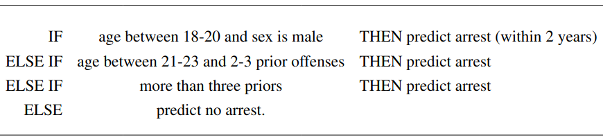
Figure 1. An example of a decision list taken from (Rudin, 2019) used to predict whether a delinquent will be arrested again. The reasoning of the decision list is directly readable.)

Feature Importance Attribution

For a given classifier and an input, feature importance attribution (FIA) or feature importance map aims to highlight what part of the input is relevant for the classifier decision on this input. The idea is that generally only a small part of the input is actually important. If for example a neural network decides whether an image contains a cat or a dog, only the part of the image displaying the respectiv animal should be considered important. This consideration omits in which way the important features were considered. It can thus be seen as the lowest level of the reasoning process.

There are quite a lot of practical approaches that derive feature importance values for neural networks, see (Mohseni et al., 2021). However, these methods are defined purely heuristically. They come without any defined target properties for the produced attributions. Furthermore, it has been demonstrated that these methods can be manipulated by clever designs of the neural network.

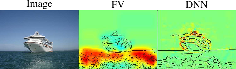
Figure 1. Feature importance map generated with LRP for a Fisher Vector Classifier (FV) and a Deep Neural Network (DNN). One can see that the FV decides the boat class based mostly on the water. Will this classifier generalise to boats without water? From (Lapuschkin et al., 2016).

Manipulation of Heuristic Feature Importance

We are talking about manipulations in the follwing sense: Given that I have a neural network classifier \(\Phi\) that performs well for my purposes, I want another classifier \(\Phi^\prime\) that performs equally well but with a completely arbitrary feature importance.

These heuristic FIAs all make implicit assumptions on the data distribution (some of them do that in a layer-wise fashion), see (Lundberg & Lee, 2017).

All these heuristic explanation methods can be manipulated with the same trick: Basically keep the on-manifold behaviour constant, but change the off-manifold behaviour to influence the interpretations.

Example from (Slack et al., 2020): \(\Phi\) is a discriminatory classifier, \(\Psi\) is a completely fair classifier and there is a helper function that decides if an input is on-manifold, belongs to a subspace of typical sample \(\mathcal{X}\). They define

Now \(\Phi^\prime\) will almost always discriminate since for \(\mathbf{x}\) that lie on the manifold, whereas the explanations will be dominated by the fair classifier \(\Psi\), since most samples for the explanations are not on manifold. Thus the FIA highlights the innocuous features instead of the discriminatory ones.

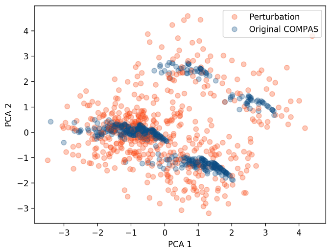
Figure 1. On-manifold data samples (blue) and off-manifold LIME-samples (red) for the COMPAS dataset; from (Dimanov et al., 2020).

Formal approaches to interpretability thus need to make the underlying data distribution explicit.

Formal definition of feature importance

There are three main approaches to feature importance attribution:

1. Shapley values
2. Prime Implicants
3. Maximal Mutual Information While Shapley values directly give a score to each feature, prime implicants and maximum mutual information select a subset of the features as the important features. However, since most search methods for these subsets work over convex relaxations of set membership, the unthresholded scores can serve as an importance value.

Shapley Values are a value attribution method from cooperative game theory. It is the unique are the unique method that satisfies the following desirable properties: linearity, symmetry, null player and efficiency (Shapley, 1997). The idea is that a set of players achieve a common value. This value is to be fairly distributed to the players according to their importance. For this one considers every possible subset of players, called a coalition and the value this coalition would achieve. Thus, to define Shapley Values one needs a so called characteristic function, a value function that is defined on a set as well as all possible subsets. For \(d\) players, let \(\nu: 2^{[d]} \rightarrow \mathbb{R}\). Then \(\phi_i\), the Shapley value of the \(i\)-th player is defined as

Thus the Shapley values sum over all marginal contributions of the \(i\)-th player for ever possible coalition. In machine learning, the players correspond to features and the coalitions to subsets of the whole input. The explicite training of a characteristic function has been used in the context of simple two-player games to compare with heuristic attribution methods in (Wäldchen et al., 2022). However, generally in machine learning, the model cannot evaluate subsets of inputs. For a given input \(\mathbf{x}\) and classification function \(f\), define \(\nu\) over expectation values:

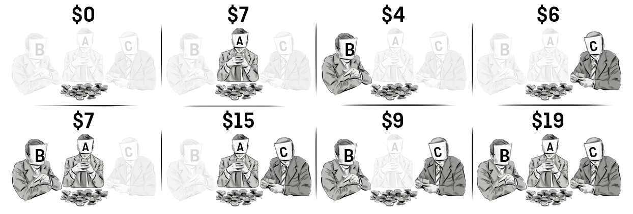
Figure 1. Illustration of the idea of Shapley Values. For three players the pay-off for each possible coalition is shown. Source

Prime Implicants

A series of appraoches considers hwo much a subset of the features of \(\mathbf{x}\) already determine the function output \(f(\mathbf{x})\). One of the most straight-forward approaches are the prime implicant explanations [D] for Boolean classifiers. An implicant is a part of the input that determines the output of the function completely, no matter which value the rest of the input takes. A prime implicant is an implicant that cannot be reduced further by omitting features.

This concept is tricky to implement for very the highly non-linear neural networks, as small parts of an input can often be manipulated to give a completely different classification, see (Brown et al., 2017). Thus, prime implicant explanations need to cover almost the whole input, and are thus not very informative.

Probabilistic prime implicants have thus be introduced. As a relaxed notion, they only require the implicant to determine the function output with some high probability \(\delta\), see (Wäldchen et al., 2021), and in (Ribeiro et al., 2018) as precision:

For continuously valued fucntions \(f\) this can be further relaxed to being close to the original value in some fitting norm. One is then often interested in the most informative subset of a given maximal size:

In the language of Shapley values, we are looking for a small coalition that already achieves a value close to the whole set of players. There is a natural trade-off between the maximal set size \(k\) and the achievable distortion \(D(S^*)\).

This concept can be refined without the arbitrariness of the norm by considering the mutual information.

Maximal Mutual Information

Mututal information measures the mutual dependence between two variables. In the context of the inpt features, it can be defined for a given subset S as as

where \(H_{\mathbf{x} \sim \mathcal{D}}[f(\mathbf{x})]\) is the a priori entropy of the classification decision and \(H_{\mathbf{x} \sim \mathcal{D}}[f(\mathbf{x}) ~|~ \mathbf{x}_S]\) is the conditional entropy given the input set. When the conditional entropy is close to zero, the mutual information takes its maximal value as the pure a priori entropy.

where \(l\) runs over the domain of \(f\). Similarly to the prime implicant explanations, one is often interested to find a small subset of the input that ensures high mutual information with the output:

The modelling Problem

All three presented methods to calculate the conditional probabilities \(\mathcal{D}_{\mathbf{x}_S}\) for all subsets \(S\) in question. For synthetic datasets these probabilities can be known, for realistic datasets however, these probabilities require explicit modelling of the conditional data distribution. This has been achieved practically with variational autoencoders or generative adversarial networks. Let us call these approximations \(\mathcal{D^\prime}|_{\mathbf{x}_S}\).

Practical Problems

There are basically two practical approaches to the modelling problem. The first is taking a simplified i.i.d. distribution (which is in particular independent of the given features):

This has been the approach taken for example in (Fong & Vedaldi, 2017),(MacDonald et al., 2019) and (Ribeiro et al., 2016). The problem here is that for certain masks this can create features that are not there in the original image, see Figure 4 for an illustration. This can actually happen even when unintended in case of an optimiser solving for small distortion \(D_{f,\mathbf{x}}\), as shown in Figure 4.

Figure 4. The optimised mask to convince the classifier of the (correct) bird class constructs a feature that is not present in the original image, here a bird head looking to the left inside of the monochrome black wing of the original; from [Macdonald2021]. This can happen because of the effect explained in Figure 5 Left.

In fact, these simplified models are the reason that the heuristic methods of LIME ans ShAP are manipulable as explained before. If they used a correct model of the data distribution, there would be no off-manifold inputs when calculating the importance valuese, and the trick to change the off-manifold behaviour of the classifier would be without effect.

The second, data-driven approach is to train a generative model on the dataset:

This has the advantage that the inpainting will likely be done more correctly thus evading the creation of new features by the mask. However, a new problem arises. Since it is likely that the classifier and the generator have been trained on the same dataset, they tend to learn the same biases which can cancel out and go undetected. An illustration is given in Figure 5 Right. The classifier learns to use water to identify ships. When a pixel mask containing the ship is selected, the generator paints the water back in, which can then be used by the classifier to answer correctly thus giving the appearance that the ship feature was used. This would give the ship high Shapley values and high mutual information, despite the classifier working in a way that will not generalise outside the dataset.

Figure 5. Different failure modes for different models of the data distribution. Both approaches have specific shortcomings. Left: Feature inpainting with an i.i.d. distribution. Selecting a mask can create a new feature that was not present in the original input. If one would consider a data-driven approach instead the rest of the image would likely be inpainted as black and the effect would disappear. Right: Data-driven inpainting. After selecting the boat feature, a trained generator inpaints the water back into the image, which the classifier uses for classification. Consequently the boat feature will get high Shaply Values/mutual information even though the classifier does not rely on boats. If one uses an i.i.d appraoch this effect would not appear.

Theoretical Problems

Since we want a formal approach with a bound on the calculated Shapley values, distortion or mutual information, we need a distance bound between \(\mathcal{D^\prime}|_{\mathbf{x}_S}\) and \(\mathcal{D}|_{\mathbf{x}_S}\) in some fitting norm, e.g. the total variation or Kullback-Leibler divergence

This is hard to achieve, since to establish such bounds one would need exponentially many samples from the dataset, since there are exponentially many subsets to condition on.

Taking any image \(\mathbf{x}\) from ImageNet for example and conditioning on a subset \(S\) of pixels, there probably exists no second image with the same values on \(S\) when size of \(S\) is larger than 20. These conditional distributions thus cannot be sampled for most high-dimensional datasets and no quality bounds can be derived. One would need to trust one trained model to evaluate another trained model — this is a very strong condition for a formal guarantee!

In the next post we discuss how this problem can be overcome by replacing the modelling of the data distribution with an adversarial setup.

◀ Previous Post

Next Post ▶

References

1. Rudin, C. (2019). Stop explaining black box machine learning models for high stakes decisions and use interpretable models instead. Nature Machine Intelligence, 1(5), 206–215.
2. Mohseni, S., Zarei, N., & Ragan, E. D. (2021). A multidisciplinary survey and framework for design and evaluation of explainable AI systems. ACM Transactions on Interactive Intelligent Systems (TiiS), 11(3-4), 1–45.
3. Lapuschkin, S., Binder, A., Montavon, G., Muller, K.-R., & Samek, W. (2016). Analyzing classifiers: Fisher vectors and deep neural networks. Proceedings of the IEEE Conference on Computer Vision and Pattern Recognition, 2912–2920.
4. Lundberg, S. M., & Lee, S.-I. (2017). A unified approach to interpreting model predictions. Advances in Neural Information Processing Systems, 30.
5. Slack, D., Hilgard, S., Jia, E., Singh, S., & Lakkaraju, H. (2020). Fooling lime and shap: Adversarial attacks on post hoc explanation methods. Proceedings of the AAAI/ACM Conference on AI, Ethics, and Society, 180–186.
6. Dimanov, B., Bhatt, U., Jamnik, M., & Weller, A. (2020). You shouldn’t trust me: Learning models which conceal unfairness from multiple explanation methods.
7. Shapley, L. S. (1997). A value for n-person games. Classics in Game Theory, 69.
8. Wäldchen, S., Pokutta, S., & Huber, F. (2022). Training characteristic functions with reinforcement learning: Xai-methods play connect four. International Conference on Machine Learning, 22457–22474.
9. Brown, T. B., Mané, D., Roy, A., Abadi Martı́n, & Gilmer, J. (2017). Adversarial patch. ArXiv Preprint ArXiv:1712.09665.
10. Wäldchen, S., Macdonald, J., Hauch, S., & Kutyniok, G. (2021). The computational complexity of understanding binary classifier decisions. Journal of Artificial Intelligence Research, 70, 351–387.
11. Ribeiro, M. T., Singh, S., & Guestrin, C. (2018). Anchors: High-precision model-agnostic explanations. Proceedings of the AAAI Conference on Artificial Intelligence, 32(1).
12. Fong, R. C., & Vedaldi, A. (2017). Interpretable explanations of black boxes by meaningful perturbation. Proceedings of the IEEE International Conference on Computer Vision, 3429–3437.
13. MacDonald, J., Wäldchen, S., Hauch, S., & Kutyniok, G. (2019). A rate-distortion framework for explaining neural network decisions. ArXiv Preprint ArXiv:1905.11092.
14. Ribeiro, M. T., Singh, S., & Guestrin, C. (2016). Model-agnostic interpretability of machine learning. ArXiv Preprint ArXiv:1606.05386.